In the previous article, we started from the CPU pipeline and looked at superscalar execution, register renaming, out-of-order issue, the ROB, and the store buffer.
The goal behind these designs is to keep different stations inside the CPU pipeline as full as possible and improve instruction throughput.
If the pipeline always has ready instructions, the ALU, load units, and store units can keep doing useful work. Conversely, when the CPU does not know what to execute next, some stages in the pipeline start to sit idle.
By identifying data dependencies, where one instruction needs the result of a previous instruction, superscalar execution and register renaming allow independent instructions to run in parallel. Out-of-order issue also prevents later independent instructions from being blocked by an earlier instruction that is still waiting.
But for superscalar execution and out-of-order execution to work well, there is an even earlier requirement: Instruction Fetch station must keep fetching new instructions without interruption.
When Does Instruction Fetch Station Stop?
Conceptually, the CPU pipeline can be roughly divided into the frontend and the backend.
The frontend is responsible for fetch, decode, rename, and preparing uops.
The backend is responsible for schedule, execute, memory access, and write back.
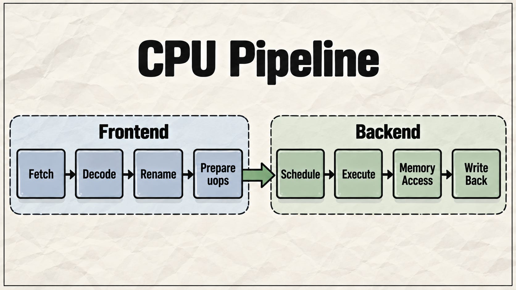
The data dependencies discussed in the previous article mainly affect the backend: if the operands of a uop are not ready, the scheduler cannot send it to an execution unit.
But another kind of dependency can block the frontend earlier: control dependency.
A control dependency means the next program counter is not yet known, so Instruction Fetch does not know where to fetch the next instruction.
Once the frontend stops, the later decode, rename, schedule, and execution units quickly run out of work. Function calls are one common source of such control dependencies.
Why Is a Function Call a Control Dependency?
Consider this code:
void f() {
  g();
  x = 1;
}

void h() {
  g();
  y = 2;

}

void g() {
  return;
}
When the CPU executes g() inside f, the call target is usually clear. In other words, the CPU knows where the code for g is. The tricky part is the return.
From the perspective of the return inside g, if g was called from f, the next instruction should go back to x = 1. If g was called from h, the next instruction should go back to y = 2.
Therefore, for Instruction Fetch, return is also a control transfer. It needs to know the return address before it can know the next PC and continue fetching.
While the CPU is waiting, the pipeline frontend may sit idle, so the compiler has a very direct optimization strategy: inline.
Inlining removes the function call and expands the callee body directly into the caller. For example, the body of g above is very small, so the compiler can expand it into f and h. Once that happens, both the call and return disappear, and the original cross-function control flow becomes a more continuous instruction stream.
Besides removing the function call, inlining also makes the callee body part of the caller. This lets the compiler continue with optimizations such as constant propagation and dead code elimination. For example:
fn add_or_sub(x: i32, add: bool) -> i32 {
    if add {
        x + 1
    } else {
        x - 1
    }
}

fn f() -> i32 {
    add_or_sub(10, true)
}
After inlining, the compiler can conceptually see:
fn f() -> i32 {
    if true {
        10 + 1
    } else {
        10 - 1
    }
}
Because add = true and x = 10 are now known constants, constant propagation plus dead code elimination can simplify the code into:
fn f() -> i32 {
  11
}
But not every function call can be inlined so easily. Object method calls are a more interesting example.
Why Can’t Object Method Calls Be Inlined Easily?
Start with a Rust trait:
trait Draw {
  fn draw(&self);
}

struct Circle;

struct Square;

impl Draw for Circle {
  fn draw(&self) {}
}

impl Draw for Square {
  fn draw(&self) {}
}
If render is written like this:
fn render<T: Draw>(x: &T) {
  x.draw();
}
And called like this:
render(&Circle);
render(&Square);
From the perspective of trait abstraction, render seems to only know that x has the Draw capability. It does not seem to know whether x is a Circle or a Square.
If the method target really had to be determined at runtime, then x.draw() would be an indirect function call, which would make it hard to inline directly.
But this version of render uses a generic type parameter plus a trait bound. In Rust, this uses static dispatch through generic monomorphization.
The compiler generates different versions of the function based on the concrete types actually used:
render(&Circle); => render_for_Circle(...) => x.draw() is Circle::draw

render(&Square); => render_for_Square(...) => x.draw() is Square::draw
Once the target becomes clear, the compiler has a chance to inline it. This is one important reason Rust generics use monomorphization: they trade more code generation for static dispatch, direct calls, and more inlining opportunities.
But Rust traits have another form that cannot be solved through monomorphization.
Why Can Rust dyn Trait Be Slower Than Generic Trait?
Traits can also be used like this:
fn render(x: &dyn Draw) {
  x.draw();
}
Here, dyn Draw means dynamic dispatch.
render does not know whether the concrete type behind x is Circle or Square. It only knows that x supports Draw.
This often appears in heterogeneous collections. For example, if an array wants to store values that all implement Draw but may actually be Circle or Square underneath, the concrete element type of Vec still has to be the same. So it is commonly declared as:
Vec<&dyn Draw> or Vec<Box<dyn Draw>>
dyn Draw is an unsized trait object type. It can be roughly understood as another object type whose fields are a data pointer and a vtable pointer:
data pointer: points to the real object, such as Circle or Square.
vtable pointer: points to a Virtual Method Table. It stores method function pointers and some metadata, and the corresponding method logic is found through a method slot id.
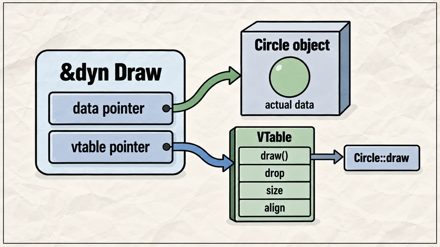
With dynamic dispatch implemented through the vtable, x.draw() conceptually executes like this:
method = x.vtable_ptr[DRAW_SLOT]

method(x.data_ptr)
Because dyn Draw is an unsized object type, it must be passed through a pointer to have a fixed size. Or it can be wrapped in Box<dyn Draw> to provide RAII, so when it leaves scope, the drop metadata in the vtable can correctly drop the concrete object pointed to by the data pointer.
Therefore, dyn Trait cannot generate render_for_Circle and render_for_Square the way generic T: Trait can. It can only call indirectly through the vtable, and usually cannot be inlined.
This is one reason dyn Trait can be slower than generic Trait.
C++ virtual methods are similar. They are usually implemented through a vtable as well. A common optimization technique is CRTP, which uses templates to implement static polymorphism.
At this point, we can see a pattern:
If the compiler knows the call target at compile time, it can use a direct call, and may even inline it. If the target is only known at runtime, the program keeps an indirect call, and the CPU frontend has to deal with the control flow.
If the Compiler Cannot Remove a Function Call, Can the CPU Optimize It by Itself?
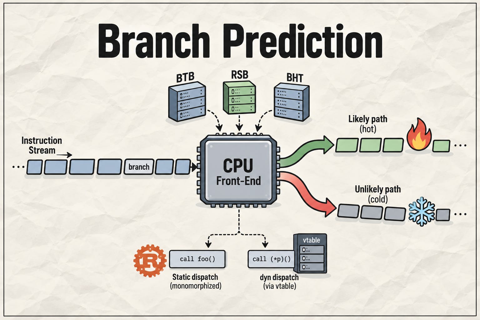
Yes. The CPU uses a hardware mechanism to predict return addresses.
This structure is called the Return Stack Buffer, or RSB. Conceptually, it is like a hardware call stack. When call g happens, the CPU pushes the address after the call into the RSB. When return happens, it pops an address from the RSB and first predicts that the return will go there.
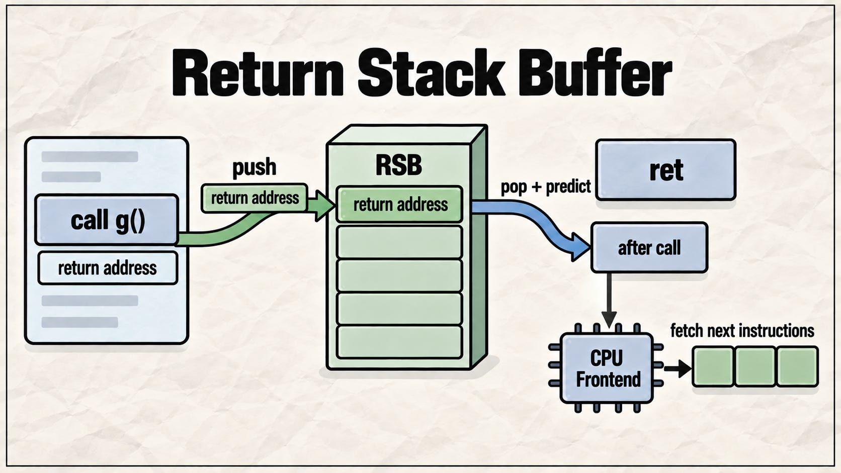
If the prediction is correct, the CPU can fetch the caller’s following instructions earlier.
If the prediction is wrong, the speculative work on the wrong path is flushed, and the CPU fetches again from the correct address. The previous work becomes wasted work.
This is part of the CPU frontend’s branch prediction mechanism. The idea of “guessing the next PC first” also appears in other control flows.
Besides Function Calls, What Other Control Flow Affects the CPU Pipeline?
The most common one is if.
if (x > 0) {
  a();
} else {
  b();
}
Conceptually, it may be compiled into:
cmp x, 0
jump_if_less_or_equal else_path
call a
jump end
else_path:
call b
end:
For the CPU to know whether the next instruction is on the a path or the b path, it first has to know the result of x > 0. To avoid leaving the pipeline idle, the CPU performs branch prediction and guesses two things:
Direction prediction: will this branch be taken or not taken?
Target prediction: if it is taken, which address should it jump to?
For example, if jump_if_less_or_equal is taken, it jumps to else_path and needs to know the instruction address of call b. If it is not taken, it does not jump and simply continues to execute the next instruction, call a.
To avoid wrong guesses, the simplest prediction method is based on past execution behavior. For example, consider a loop branch:
for (int i = 0; i < 4; i++) {
  work();
}
After compilation:
loop_start:
work()
i = i + 1
cmp i, 4
jump_if_less loop_start
If the jump_if_less branch is taken, it returns to loop_start. If it is not taken, execution falls through and breaks out of the loop. The simplest predictor can use 1 bit to record branch history:
The 1st to 3rd times (i: 0 to 2) are all Taken. The 4th time (i: 3) can still be predicted as Taken, so Instruction Fetch can fetch work() without waiting for the jump_if_less result. But on the 5th time (i: 4), if it still predicts Taken, it will be wrong. At this point, the branch history is:
T T T T N
When the same loop runs a second time, the previous failure leaves the predictor state at N. The CPU follows the previous state and predicts N, so it gets the first iteration wrong again. The optimization is to use a 2-bit state machine:
Strongly Taken (ST), Weakly Taken (WT), Weakly Not Taken (WN), and Strongly Not Taken (SN).
During the first loop, the state sequence is WT ST ST ST WT. When WT sees one wrong prediction, it only moves to WN if it is wrong again, so the second execution of the loop still predicts Taken. The second loop then becomes ST ST ST ST WT. This means only the final round of each loop is mispredicted, reducing repeated loop mispredictions from 2*n+1 to n.
More advanced CPUs use a loop predictor to remember the taken and not-taken counts of this loop. For example, after observing this loop:
T T T T N
The next time, it can predict:
the first four times are taken, and the fifth time is not taken and exits the loop. If the iteration count is stable, the loop predictor can even correctly predict the final exit.
But this iteration-count-based predictor is suitable for loops because loop branch behavior has a clear direction: Taken states are usually consecutive. Other control flow, such as if-else, does not necessarily have this property.
How Does a Normal if-else Use History for Prediction?
A normal if branch often depends on runtime data. For example:
if (x > 0) {
  a();
} else {
  b();
}
If x comes from a request, the branch result may not have a fixed iteration count. In this case, the predictor uses branch history and patterns.
A simplified model is:
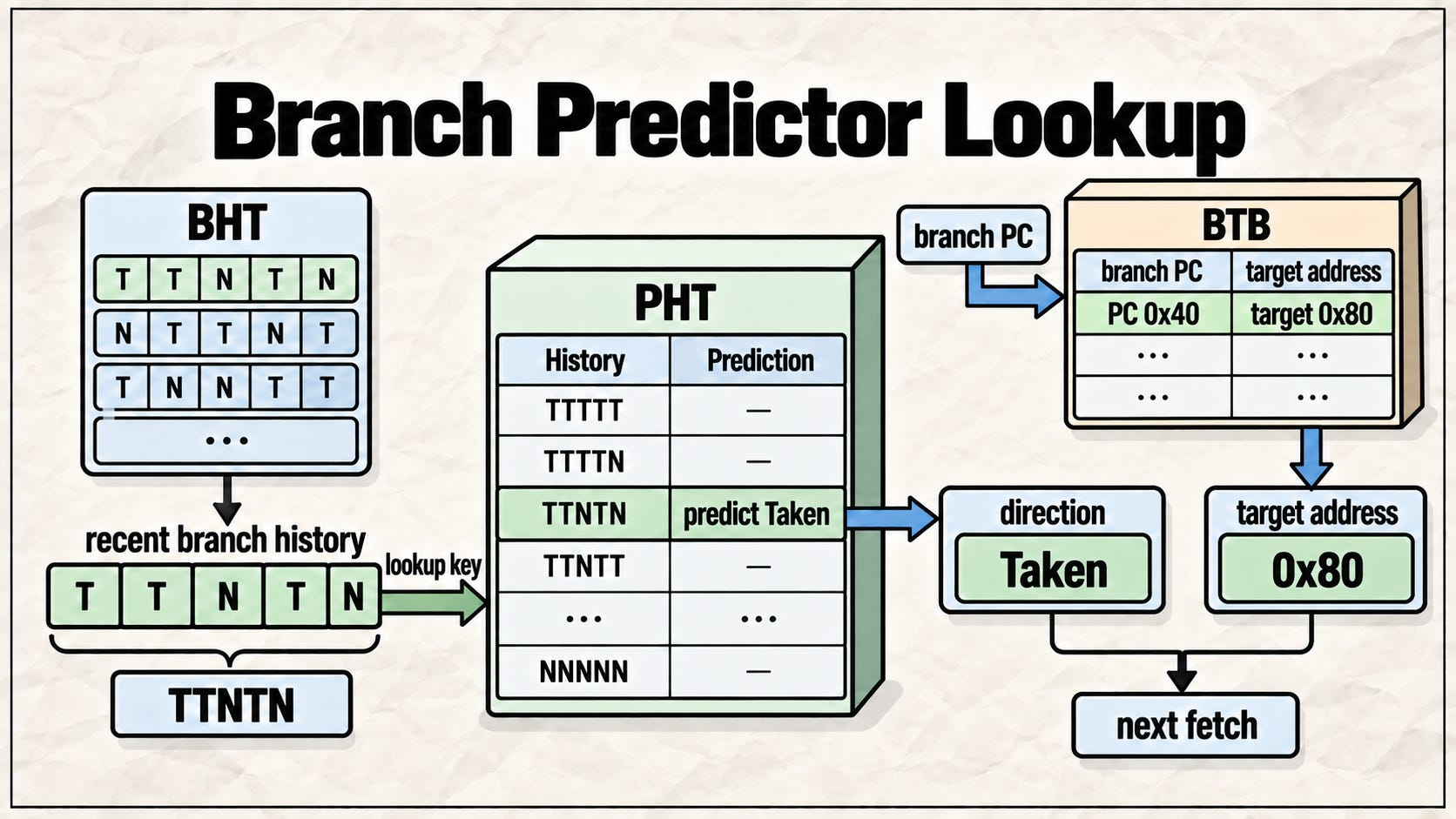
The CPU records the recent results of a branch, such as:
T T N T N
It uses this history, TTNTN, as a key to look up a predictor table and find the likely next state. Therefore, branch prediction has two tables:
BHT, Branch History Table, records branch history.
PHT, Pattern History Table, records the likely next state for a given history pattern.
BTB, Branch Target Buffer, records which instruction address a branch should jump to if it is taken.
In real programs, different branches are often correlated. For example:
if (req.method == POST) {
  ...
}

if (req.body_bytes > 0) {
 ...
}
When `req.method is POST, req.body_bytes > 0 is also more likely to be true. Therefore, the predictor can look not only at a branch’s own local history, but also at the global history of recent branches. For example, T T N T N can represent the states of the previous five branches. In simple terms:
Local history stores how this specific branch behaved in the past, while global history stores what the recent overall control flow looked like.
Modern CPU branch predictors combine many information sources, such as local history and global history, to improve accuracy. But prediction is not free. It requires additional hardware space for RSB, history, and predictor state, and it also requires extra table lookups and selection logic.
And even if prediction is usually accurate, one wrong guess can turn fetched, decoded, renamed, and even partially executed work on the wrong path into wasted work.
Therefore, the compiler still needs to optimize control flow.
How Does the Compiler Help Control Flow Run Faster?
The most direct optimization is similar to inlining a function call away: sometimes the compiler can eliminate a branch jump through branchless transformation.
For example, suppose x is dynamically determined by a request:
if (x > 10) {
  count += 1;
}
Conceptually, after compilation this may become:
cmp x, 10
jump_if_less_or_equal skip
add count, 1
skip:
When jump_if_less_or_equal is hard to predict, the CPU may often put instructions from the wrong path into the pipeline, causing wasted work. In this case, the compiler can transform it into:
count += (x > 10);Conceptually, it becomes:
cmp x, 10
flag = condition ? 1 : 0
add count, flag
Now the jump_if_less_or_equal branch disappears. There is no branch jump to predict. But set flag still depends on the result of cmp x, 10, so the dependency has not disappeared. It has only changed from a control dependency into a data dependency. The instruction stream can now continue forward without a jump and without guessing the next PC.
The tradeoff is that branchless code often has to prepare the values for both outcomes first, such as 1 and 0, and then select or combine the right one afterward.
Therefore, branchless code is suitable for small value selection, such as adding 0 or 1 to count, or operations like max(a, b). But branchless transformation is not universal. For example:
if (req.is_premium) {
  handle_premium();
} else {
  handle_normal();
}
handle_premium and handle_normal may contain complex logic. You would not want to execute both handle_premium and handle_normal first and then choose one result. In this case, besides relying on the CPU predictor, the compiler’s machine-instruction layout also matters.
The example above can be arranged in two shapes.
case A:
cmp req.is_premium, true
jump_if_false normal
handle_premium
return
normal:
handle_normal
return
case B:
cmp req.is_premium, true
jump_if_true premium
handle_normal
return
premium:
handle_premium
return
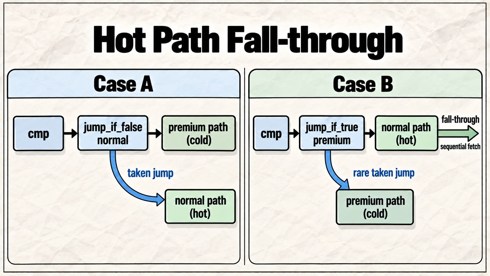
Assume req.is_premium is rare. Then handle_normal is the hot path, and handle_premium is the cold path.
In case A, the jump_if_false normal branch is frequently taken and jumps to normal. Since instructions are laid out sequentially in the instruction cache, a jump redirect makes the instruction stream less sequential and less continuous, which may reduce instruction locality.
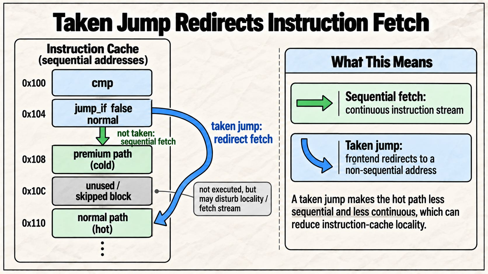
Therefore, case B is the better layout. jump_if_true premium is usually not taken, so the instruction stream can be fetched sequentially and naturally reach the normal path.
This is hot path fall-through optimization. It does not eliminate the branch. It makes the most common path correspond to “do not jump, just continue executing downward.”
How Does the Compiler Know Which Path Is Hot?
The first source is heuristics plus programmer hints. Based on experience, panic paths, throw paths, bounds-check failures, and error paths are usually not triggered often, so they can be marked as cold paths to tell the compiler.
For Rust’s unwrap, conceptually it looks like this:
#[inline(always)]
pub const fn unwrap(self) -> T {
    match self {
        Some(val) => val,
        None => unwrap_failed(),
    }
}

#[cfg_attr(not(panic = “immediate-abort”), inline(never))]
#[cold]
#[track_caller]
const fn unwrap_failed() -> ! {
    panic(”called `Option::unwrap()` on a `None` value”)
}
The #[cold] attribute tells the compiler that this is a cold path, allowing the compiler to lay out code more appropriately. C++ also has [[likely]] and [[unlikely]].
The second source is Profile-Guided Optimization, or PGO. First, an instrumented binary is run with a real workload to collect which branches are common, which functions are hot, and which blocks are cold. Then the program is recompiled using that profile. This is more reliable than manually guessing the hot path because it uses actual execution data.
For example, Rust can use LLVM PGO. Besides hot path marking, if the profile shows that a dyn Trait is almost always one concrete type, the compiler may optimize that concrete type into a direct dispatch plus inline fast path:
fn render(x: &dyn Draw) {
    // Original:
    // call x.vtable.draw(x.data)
    // PGO finds that most cases use Circle as the concrete type.

    if likely_is_circle(x) {
        Circle::draw(x.data)   // direct call, possibly inline
    } else {
        x.vtable.draw(x.data)  // fallback dynamic dispatch
    }
}
Other Interesting Branch-Related Compiler Optimizations
The first one is bounds check elimination.
For example:
sum += slice[i];This actually contains a condition check: if i is out of bounds, the program has to panic.
But if the code is:
for i in 0..slice.len() {
  sum += slice[i];
}
The compiler may be able to prove that i is always between 0 and slice.len(), so it does not need to perform a bounds check every time. It can directly remove that unnecessary branch.
The second one is loop unswitching.
Suppose we have:
for (int i = 0; i < n; i++) {
  if (debug) {
    slow_debug(a[i]);
  } else {
    fast(a[i]);
  }
}
If debug does not change throughout the loop, the original code has to check debug every iteration.
The compiler can transform it into:
if (debug) {
  for (int i = 0; i < n; i++) {
    slow_debug(a[i]);
  }
} else {
  for (int i = 0; i < n; i++) {
    fast(a[i]);
  }
}
This moves the debug branch from inside the loop to outside the loop. The branch only runs once before entering the loop, reducing the number of branch predictions. The loop body also becomes simpler, making it easier for the compiler to perform loop unrolling.
Summary
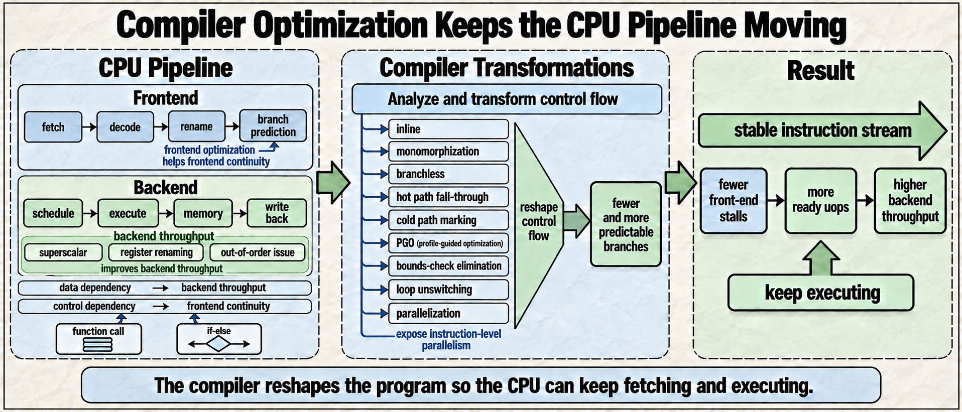
The CPU pipeline can be divided into the frontend (fetch, decode, rename) and the backend (schedule, execute, memory access, write back). The superscalar execution, register renaming, and out-of-order issue discussed in the previous article are mainly about improving backend throughput.
But backend throughput can only improve if frontend throughput also keeps up. The key issue for backend throughput is data dependency, while the key issue for the frontend is control dependency, such as function calls and if-else.
From the perspective of CPU architecture, compiler optimization often helps the CPU keep the instruction stream stable. Inlining removes function calls and returns. Rust generics use monomorphization to turn trait method calls into static dispatch, increasing opportunities for direct calls and inlining.
When a branch cannot be eliminated, the CPU uses branch prediction to guess the next PC. The compiler uses techniques such as branchless transformation, hot path fall-through, cold path marking, PGO, bounds check elimination, and loop unswitching to make control flow easier to predict or less frequent.
The core idea is simple: the compiler is not just making code shorter. It is reshaping the program into a form that is easier for the CPU pipeline to keep executing.